Defining the film
We first need to define the materials
from refl1d.names import *
from copy import copy

# === Materials ===
SiOx = SLD(name="SiOx", rho=3.47)
D_toluene = SLD(name="D-toluene", rho=5.66)
D_initiator = SLD(name="D-initiator", rho=1.5)
D_polystyrene = SLD(name="D-PS", rho=6.2)
H_toluene = SLD(name="H-toluene", rho=0.94)
H_initiator = SLD(name="H-initiator", rho=0)
In this case we are using the neutron scattering length density as is
standard practice in reflectivity experiments rather than the chemical
formula and mass density. The SLD class
allows us to name the material and define the real and imaginary components
of scattering length density \(\rho\). Note that we are using the imaginary
\(\rho_i\) rather than the absorption coefficient \(\mu = 2\lambda\rho_i\)
since it removes the dependence on wavelength from the calculation of
the reflectivity.
For the tethered polymer we don’t use a simple slab model, but instead
define a PolymerBrush
layer, which understands that the system is compose of polymer plus
solvent, and that the polymer chains tail off like:
This volume profile combines with the scattering length density of the polymer and the solvent to form an SLD profile:
The tethered polymer layer definition looks like
# === Sample ===
# Deuterated sample
D_brush = PolymerBrush(polymer=D_polystyrene, solvent=D_toluene, base_vf=70, base=120, length=80, power=2, sigma=10)
This layer can be combined with the remaining layers to form the deuterated measurement sample
D = silicon(0, 5) | SiOx(100, 5) | D_initiator(100, 20) | D_brush(400, 0) | D_toluene
The stack notation material(thickness, interface) | ... is performing
a number of tasks for you. One thing it is doing is wrapping materials
(which are objects that understand scattering length densities) into
slabs (which are objects that understand thickness and interface). These
slabs are then gathered together into a stack:
L_silicon = Slab(material=silicon, thickness=0, interface=5)
L_SiOx = Slab(material=SiOx, thickness=100, interface=5)
L_D_initiator = Slab(material=D_initiator, thickness=100, interface=20)
L_D_brush = copy(D_brush)
L_D_brush.thickness = Parameter.default(400, name=D_brush.name+" thickness")
L_D_brush.interface = Parameter.default(0, name=D_brush.name+" interface")
L_D_toluene = Slab(material=D_toluene)
D = Stack([L_silicon, L_SiOx, L_D_initiator, L_D_brush, L_D_toluene])
The undeuterated sample is similar to the deuterated sample. We start by copying the polymer brush layer so that parameters such as length, power, etc. will be shared between the two systems, but we replace the deuterated toluene solvent with undeuterated toluene. We then use this H_brush to define a new stack with undeuterated tolune
# Undeuterated sample is a copy of the deuterated sample
H_brush = copy(D_brush)  # Share tethered polymer parameters...
H_brush.solvent = H_toluene  # ... but use different solvent
H = silicon | SiOx | H_initiator | H_brush | H_toluene
We want to share thickness and interface between the two systems as well, so we write a loop to go through the layers of D and copy the thickness and interface parameters to H
for i, _ in enumerate(D):
    H[i].thickness = D[i].thickness
    H[i].interface = D[i].interface
What is happening internally is that for each layer in the stack we are copying the parameter for the thickness from the deuterated sample slab to the thickness slot in the undeuterated sample slab. Similarly for interface. When the refinement engine sets a new value for a thickness parameter and asks the two models to evaluate \(\chi^2\), both models will see the same thickness parameter value.
Setting fit ranges
With both samples defined, we next specify the ranges on the fitted parameters
# === Fit parameters ===
for i in (0, 1, 2):
    D[i].interface.range(0, 100)
D[1].thickness.range(0, 200)
D[2].thickness.range(0, 200)
D_polystyrene.rho.range(6.2, 6.5)
SiOx.rho.range(2.07, 4.16)  # Si to SiO2
D_toluene.rho.pmp(5)
D_initiator.rho.range(0, 1.5)
D_brush.base_vf.range(50, 80)
D_brush.base.range(0, 200)
D_brush.length.range(0, 500)
D_brush.power.range(0, 5)
D_brush.sigma.range(0, 20)

# Undeuterated system adds two extra parameters
H_toluene.rho.pmp(5)
H_initiator.rho.range(-0.5, 0.5)
Notice that in some cases we are using layer number to reference the
parameter, such as D[1].thickness whereas in other cases we are using
variables directly, such as D_toluene.rho. Determining which to
use requires an understanding of the underlying stack model. In this
case, the thickness is associated with the SiOx slab thickness, but
we never formed a variable to contain Slab(material=SiOx), so we
have to reference it via the stack. We did however create a variable
to contain Material(name="D_toluene") so we can access its parameters
directly. Also, notice that we only need to set one of D[1].thickness
and H[1].thickness since they are the same underlying parameter.
Attaching data
Next we associate the reflectivity curves with the samples:
# === Data files ===
instrument = NCNR.NG7(Qlo=0.005, slits_at_Qlo=0.075)
D_probe = instrument.load("10ndt001.refl", back_reflectivity=True)
H_probe = instrument.load("10nht001.refl", back_reflectivity=True)

D_probe.theta_offset.range(-0.1, 0.1)
We set back_reflectivity=True because we are coming in through the
substrate. The reflectometry calculator will automatically reverse
the stack and adjust the effective incident angle to account for the
refraction when the beam enters the side of the substrate. Ideally
you will have measured the incident beam intensity through the substrate
as well so that substrate absorption effects are corrected for in your
data reduction steps, but if not, you can set an estimate for
back_absorption when you load the file. Like intensity you can
set a range on the value and adjust it during refinement.
Finally, we define the fitting problem from the probes and samples. The dz parameter controls the size of the profiles steps when generating the tethered polymer interface. The dA parameter allows these steps to be joined together into larger slabs, with each slab having \((\rho_{\text max} - \rho_{\text min}) w < \Delta A\).
# === Problem definition ===
D_model = Experiment(sample=D, probe=D_probe, dz=0.5, dA=1)
H_model = Experiment(sample=H, probe=H_probe, dz=0.5, dA=1)
models = H_model, D_model
This is a multifit problem where both models contribute to the goodness of fit measure \(\chi^2\). Since no weight vector was defined the fits have equal weight.
problem = FitProblem(models)
problem.name = "tethered"
The polymer brush model is a smooth profile function, which is evaluated
by slicing it into thin slabs, then joining together similar slabs to
improve evaluation time. The dz=0.5 parameter tells us that we
should slice the brush into 0.5 Å steps. The dA=1 parameter
says we should join together thin slabs while the scattering density
uncertainty in the joined slabs \(\Delta A < 1\), where
\(\Delta A = (\max\rho - \min\rho)(\max z - \min z)\). Similarly for
the absorption cross section \(\rho_i\) and the effective magnetic cross
section \(\rho_M \cos(\theta_M)\). If dA=None (the default) then no
profile contraction occurs.
The resulting model looks like:

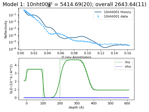
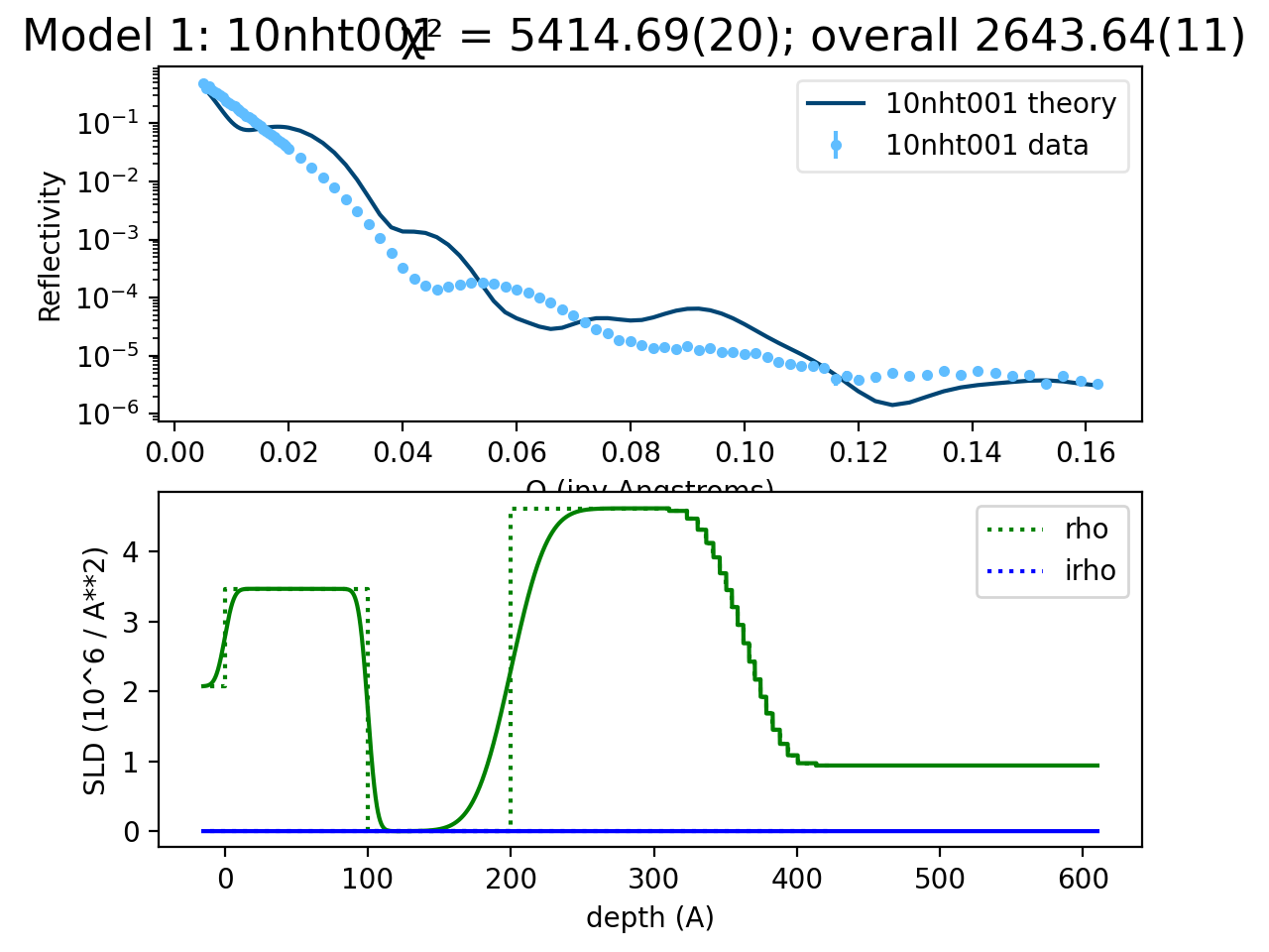

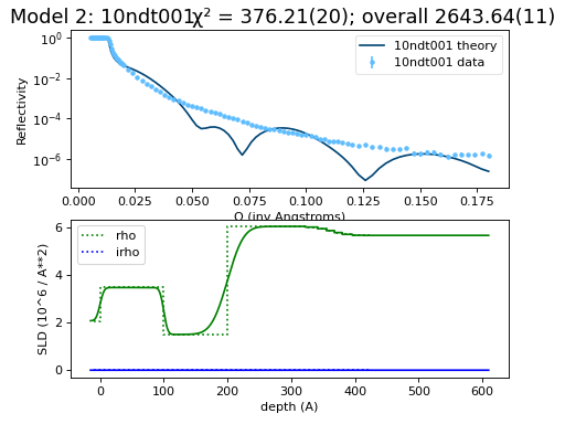
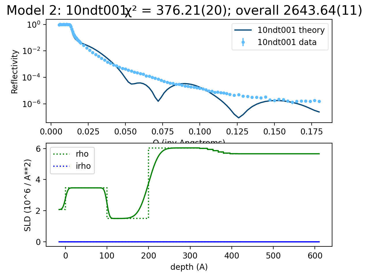
This complete model script is defined in
tethered.py:
from refl1d.names import *
from copy import copy

# === Materials ===
SiOx = SLD(name="SiOx", rho=3.47)
D_toluene = SLD(name="D-toluene", rho=5.66)
D_initiator = SLD(name="D-initiator", rho=1.5)
D_polystyrene = SLD(name="D-PS", rho=6.2)
H_toluene = SLD(name="H-toluene", rho=0.94)
H_initiator = SLD(name="H-initiator", rho=0)

# === Sample ===
# Deuterated sample
D_brush = PolymerBrush(polymer=D_polystyrene, solvent=D_toluene, base_vf=70, base=120, length=80, power=2, sigma=10)

D = silicon(0, 5) | SiOx(100, 5) | D_initiator(100, 20) | D_brush(400, 0) | D_toluene

# Undeuterated sample is a copy of the deuterated sample
H_brush = copy(D_brush)  # Share tethered polymer parameters...
H_brush.solvent = H_toluene  # ... but use different solvent
H = silicon | SiOx | H_initiator | H_brush | H_toluene

for i, _ in enumerate(D):
    H[i].thickness = D[i].thickness
    H[i].interface = D[i].interface

# === Fit parameters ===
for i in (0, 1, 2):
    D[i].interface.range(0, 100)
D[1].thickness.range(0, 200)
D[2].thickness.range(0, 200)
D_polystyrene.rho.range(6.2, 6.5)
SiOx.rho.range(2.07, 4.16)  # Si to SiO2
D_toluene.rho.pmp(5)
D_initiator.rho.range(0, 1.5)
D_brush.base_vf.range(50, 80)
D_brush.base.range(0, 200)
D_brush.length.range(0, 500)
D_brush.power.range(0, 5)
D_brush.sigma.range(0, 20)

# Undeuterated system adds two extra parameters
H_toluene.rho.pmp(5)
H_initiator.rho.range(-0.5, 0.5)

# === Data files ===
instrument = NCNR.NG7(Qlo=0.005, slits_at_Qlo=0.075)
D_probe = instrument.load("10ndt001.refl", back_reflectivity=True)
H_probe = instrument.load("10nht001.refl", back_reflectivity=True)

D_probe.theta_offset.range(-0.1, 0.1)

# === Problem definition ===
D_model = Experiment(sample=D, probe=D_probe, dz=0.5, dA=1)
H_model = Experiment(sample=H, probe=H_probe, dz=0.5, dA=1)
models = H_model, D_model

problem = FitProblem(models)
problem.name = "tethered"
The model can be fit using the parallel tempering optimizer:
$ refl1d tethered.py --fit=pt --store=T1