Soft material structures
Inter-diffusion properties of multilayer systems are of great interest in both hard and soft materials. Jomaa, et. al have shown that reflectometry can be used to elucidate the kinetics of a diffusion process in polyelectrolytes multilayers. Although the purpose of this paper was not to fit the presented system, it offers a good model for an experimentally relevant system for which information from neutron reflectometry can be obtained. In this model system we will show that we can create a model for this type of system and determine the relevant parameters through our optimisation scheme. This particular example uses deuterated reference layers to determine the kinetics of the overall system.
Reference: Jomaa, H., Schlenoff, Macromolecules, 38 (2005), 8473-8480 http://dx.doi.org/10.1021/ma050072g
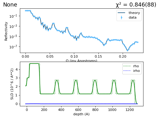
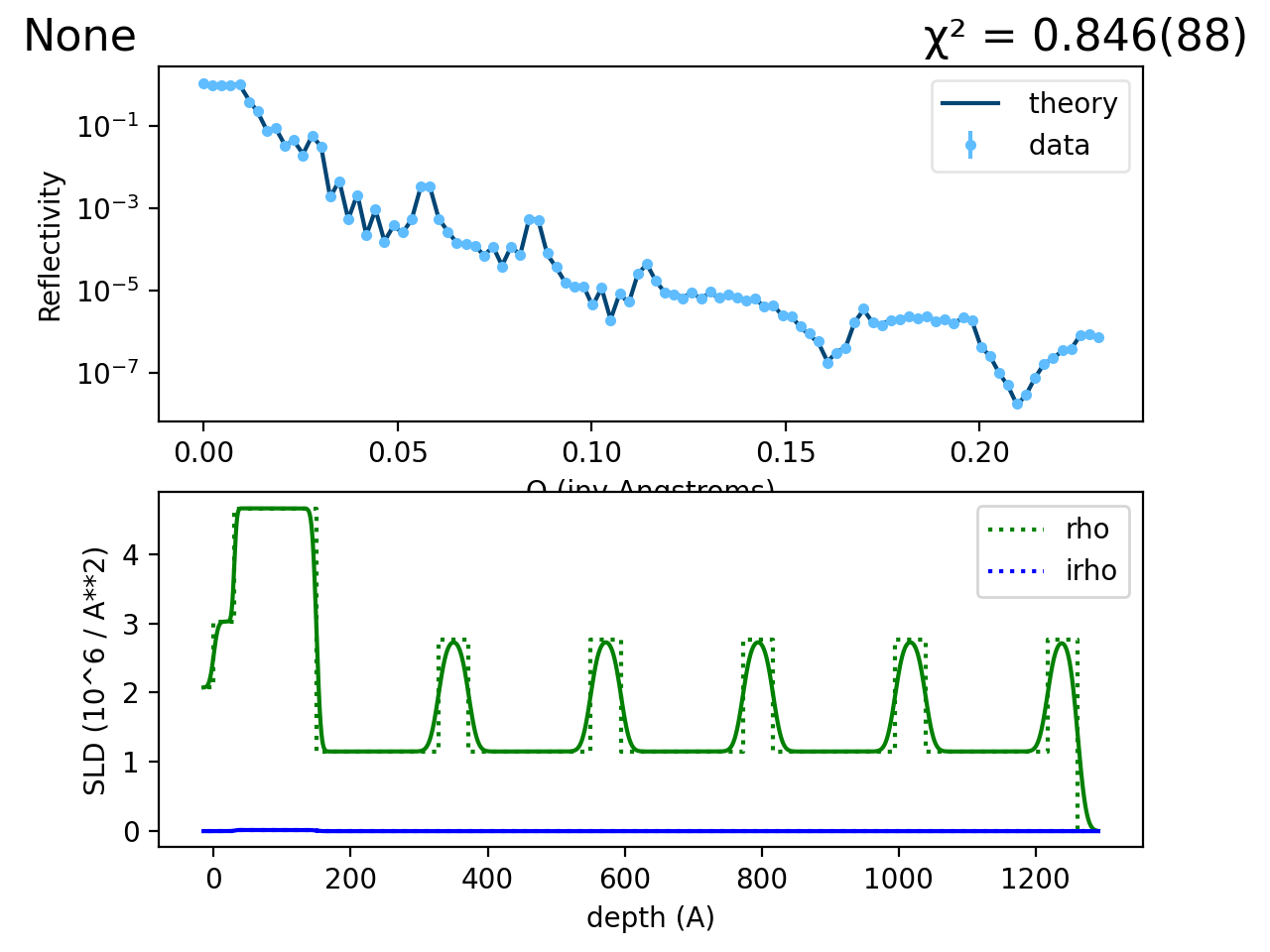
We will model the system described in figure 2 of the reference as
PEMU.py.
(Source code, png, hires.png, pdf)

Bring in all of the functions from refl1d.names so that we can use them in the remainder of the script.
import numpy

from refl1d.names import *
The polymer system is deposited on a gold film with chromium as an adhesion layer. Because these are standard films which are very well-known in this experiment we can use the built-in materials library to create these layers.
# == Sample definition ==
chrome = Material("Cr")
gold = Material("Au")
The polymer system consists of two polymers, deuterated and non-deuterated PDADMA/PSS. Since the neutron scattering cross section for deuterium is considerably different from that for hydrogen while having nearly identical chemical properties, we can use the deuterium as a tag to see to what extent the deuterated polymer layer interdiffuses with an underated polymer layer.
We model the materials using scattering length density (SLD) rather than using the chemical formula and mass density. This allows us to fit the SLD directly rather than making assumptions about the specific chemical composition of the mixture.
PDADMA_dPSS = SLD(name="PDADMA dPSS", rho=2.77)
PDADMA_PSS = SLD(name="PDADMA PSS", rho=1.15)
The polymer materials are stacked into a bilayer, with thickness estimates based on ellipsometery measurements (as stated in the paper).
bilayer = PDADMA_PSS(178, 10) | PDADMA_dPSS(44.3, 10)
The bilayer is repeated 5 times and stacked on the chromium/gold substrate In this system we expect the kinetics of the surface diffusion to differ from that of the bulk layer structure. Because we want the top bilayer to optimise independently of the other bilayers, the fifth layer was not included in the stack. If the diffusion properties of each layer were expected to vary widely from one-another, the repeat notation could not have been used at all.
sample = (
    silicon(0, 5) | chrome(30, 3) | gold(120, 5) | (bilayer) * 4 | PDADMA_PSS(178, 10) | PDADMA_dPSS(44.3, 10) | air
)
Now that the model sample is built, we can start adding ranges to the fit parameters. We assume that the chromium and gold layers are well known through other methods and will not fit it; however, additional optimisation could certainly be included here.
As stated earlier, we will be fitting the SLD of the polymers directly. The range for each will vary from that for pure deuterated to the pure undeuterated SLD.
# == Fit parameters ==
PDADMA_dPSS.rho.range(1.15, 2.77)
PDADMA_PSS.rho.range(1.15, 2.77)
We are primarily interested in the interfacial roughness so we will fit those as well. First we define the interfaces within the repeated stack. Note that the interface for bilayer[1] is the interface between the current bilayer and the next bilayer. Here we use sample[3] as the repeated bilayer, which is the 0-origin index of the bilayer in the stack.
sample[3][0].interface.range(5, 45)
sample[3][1].interface.range(5, 45)
The interface between the stack and the next layer is controlled from the repeated bilayer.
sample[3].interface.range(5, 45)
Because the top bilayer has different dynamics, we optimize the interfaces independenly. Although we want the optimiser to threat these parameters independently because surface diffusion is expected to occur faster, the overall nature of the diffusion is expected to be the same and so we use the same limits.
sample[4].interface.range(5, 45)
sample[5].interface.range(5, 45)
Finally we need to associate the sample with a measurement. We do not have the measurements from the paper available, so instead we will simulate a measurement but setting up a neutron probe whose incident angles range from 0 to 5 degrees in 100 steps. The simulated measurement is returned together with the model as a fit problem.
# == Data ==
T = numpy.linspace(0, 5, 100)
probe = NeutronProbe(T=T, dT=0.01, L=4.75, dL=0.0475)

M = Experiment(probe=probe, sample=sample)
M.simulate_data(5)

problem = FitProblem(M)